Sunday, December 28, 2014

The MV=PQ Path to the MGB Monetary Base

The Fiscal Theory of Price Level uses a monetary base to build a model predicting future prices. The available measures of money supply may not be the best measures to use. This post will explore the possibility that total government borrowing may be a good measure of money supply.

Income equals expense. This simple accounting identity underlays all economic trade. It expresses in mathematical form the concept that property is traded for property. The identity is true for both traders, only the direction is reversed.

It is important to this discussion to be aware that income and expense are considered to have occurred over some time period. The length of the time period is unspecified but is usually on a year-to-year basis. Notice that the equation stands alone without interaction between the time periods, a fact that we will overcome later in the discussion.

We can use the 'income equals expense' identity in macroeconomics by writing M*V = P*Q. [1] The left side of the equation can be considered as a general expression of income. The right side is the data driven value of all prices and quantities traded, considered as expenses.

On the income side, the term M (Money supply) represents a master supply of money available during the data period.  The master supply of money can be measured with M1, M2, and MZM, terms often associated with the quantity theory of money .  We will look for another way to measure money supply, a measure linked to past prices and quantities.

Establish Government Borrowing as a Stable Feature of the Macro-economy. [2]

We begin by using M*V = P*Q  to take a better look at the private economy, keeping in mind that we are looking for another measure of money supply.

Assume that M*V = P*Q = GDP (Gross Domestic Product) as measured by Federal Reserve statistics. We can then write for the macro-economy

GDP = GDP

which gives us an expression for macro-trade where income equals expenses.

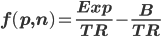
We will find the private sector GDP (PGDP) by subtracting the government sector. If we used the government budget constraint components Expense (Exp) = Taxes (T) + Borrowing (B), the result of the subtraction would be

GDP - Exp = GDP - T - B                                (1)

giving us an expression of private economy activity defined in two ways. It would also be correct to write

PGDP = GDP - Exp = GDP - T - B.                (2)

This identity becomes troubling because many economist will deny that the B term is money. They would be right. The term B is borrowing recorded in amount equal to an identical amount spent to pay government expenses. Despite having a non-money status, the B term must represent new money created in a manner similar to money creation by bank lending (A loan note is traded for money, the money is spent to form new bank deposits, and only the note remains as evidence of the trade)

Equation (2) reveals that term B must carry between measuring periods. Stated another way, borrowing not paid in one period would continue into the next period. This would be an important consideration in any model of the economy that spanned between time periods. This delayed purchasing power is in addition to the purchasing power represented by all the deposits created by government spending. Stated another way, government borrowing measures BOTH outstanding money and delayed purchasing power.

When we look at the historical record for the United States, we see that the national budget has been in deficit for nearly all the years since the 1930s. The sum of all the borrowing has reached a number that nearly matches the size of annual GDP. It is reasonable to consider that the debt can be used as a measure of monetary base, with some fraction of the base constantly available in a form of the commonly exchanged property money.

Government borrowing has been described as a stable record of money creation which would make the record a suitable monetary base. We will label the government borrowing monetary base as MGB.

This base recognition would agree with concepts from Modern Monetary Theory (MMT) as expressed by Randall Wray, Joseph Laliberte and many others. (Laliberte's post delves into the use of M*V = P*Q as a vehicle for monetary policy.)

Comparing M2 and the Sum of Government Borrowing MGB

As we go boldly into the realm of a new money supply measure, we need to compare the well accepted measures with the new. We will look at M2 as an example remembering that M1 and MZM have similar underpinnings.

The most notable characteristic of all three measures of money supply is that they are all bank based. That is, the amount of money on deposit in banks is an important component of each measure. This has an inherent problem because bank loans create the illusion of increased money supply as described previously. The central bank can reduce the visible amount by exchanging bonds for currency (some would say 'reserves'). M2 is one measure of the remaining money supply left in banks.

Chart 1 is a comparison of the actual values of M2 and government borrowing MGB. [3] The reader can see that the two values are roughly the same and follow roughly the same trajectory. Why would the two measurements follow roughly the same trajectory? Because they both attempt to measure a base money supply.

Chart 1. M2 and MGB. MGB is "Federal Debt Held by the Public" FYGFDPUN .
Economic theoreticians need a stable reference platform. From Chart 1, M2 looks more stable as it traces a gentle curve across the chart. We will consider if this is a result of central bank activity after looking at the next chart.

 We will compare private sector GDP  (PGDP) vigor with the ratio of pricing to money supply, which is commonly called velocity. We use two measures of money supply, M2 and MGB as the reference scale. Velocity is the balancing term plotted in Chart 2.

Chart 2. Private GDP velocity vs M2 and MGB. MGB is the longer trace. [3]
The velocity trace for M2 is dramatically different from the MGB trace. This is not surprising if we consider that M2 is the result of adjustments by the monetary authority. The peaks in MGB velocity would be a reflection of the large volume of bank borrowing during the peak years. The increase bank borrowing barely shows on the M2 velocity trace.

Chart 2 illustrates the difficulties a theorist would have when using either money supply measurement as a stable base. MGB has an advantage that the value of borrowing is driven by fiscal policy and is recorded as a matter of accounting. M2 would need an adjustment term to account for delayed purchasing power if it was used in a model.

MGB can be as stable as the government desires. It will increase or decrease at the rate of change in government deficits.

Conclusion

In Chart 2, the rate of annual money turnover (MGB) is seen to have declined as the supply has grown. This is an indication that prices are not directly related to money supply.

A trend line can be drawn along the bottom of the peaks. The peaks seem to correspond to periods of high construction activity which can be seen to have lasted for several years. This may be the result of higher rates of bank borrowing activity, a possibility that would be worthy of further study.

Note [1]. M*V = P*Q is a widely used equation associated with the quantity theory of money . Money Supply (M) times Velocity (V) equals Price (P) times Quantity (Q). Velocity and Quantity both are scales measured in number of transactions. Money Supply and Price both are scales measured in price per transaction. The quantity theory postulates that a change in the money scale will drive a change in the price scale. In this post, the equation is used in a different way.

Note [2]. A relationship between government borrowing and money supply is found in a different way in the post "Suggestions for Enhancement of Modern Monetary Theory (MMT)".

Note [3]. The Federal Reserve has provided the data series "Federal Debt Held by the Public" FYGFDPUN which seems to capture the sum of all Federal borrowing. FYGFDPUN seems to be the sum of Federal Reserve series FDHBFRBN and FDHBPIN, identical except for scale.

(c) Roger Sparks 2014

Sunday, December 21, 2014

Suggestions to Enhance the Modern Monetary Theory (MMT)

Modern Monetary Theory (MMT) has a widely accepted basic premise: Government can print all the money it wishes. If we accept this, the theory should then map the pathway used for entry of new money into the economy.

MMT skeptics immediately point out that if government did print at will, the money would immediately have no value. The reply by MMT supporters is that value is provided by government taxation. People, they seem to say, work to pay their taxes. This is not a satisfying reply.

In this post, we will find a more satisfying explanation for the initial value of fiat money. We will also develop an equation and map for creating a money supply and bringing it into the economy. We will begin with the equation because the method of money creation is important to the initial valuation.

Developing an equation for money creation

An equation will be built from the widely used government budget accounting constraint "expense equals income", This can be restated as "government expenses (Exp) are met by taxation (T) and borrowing (B)" and written as

    Exp = T + B.                                           (1)

Government can only tax the bigger private economy. (If there is no private economy, there is nobody to tax.) We will assume that government levies a tax on private economic transactions at a tax rate TR. The private economy is big and diverse so we will use a very general math function f(p, n) as the representative term [p is price, n is number of taxable transactions]. The private economy taxation can be  described as T = TR * f(p,n).

We will substitute the public terms into equation (1) to get

    Exp = TR * f(p,n) + B.                          (2)

Equation (2) binds government as an entity to the entire private economy. This equation would be correct over all periods of time, long or short.

Finally, to arrive at an equation explaining how money is created by government, we rearrange equation (2) to write

                                  (3)

In the simple accounting view, this equation has little to offer. In the MMT view, this equation explains how money is created. We will break it down from the MMT viewpoint.

The term Exp / TR is the normal purchase of labor and property using existing money. The term TR is a proportional vehicle. [Note 1]

The second term B / TR is puzzling and needs additional explanation. The term is preceded by a negative sign that indicates that borrowing subtracts from the payment of expenses. This means that borrowing has been used for payment but in reality, payment for expenses has not yet occurred. Instead, a promise to pay has been issued.

Equation (3) indicates that the private economy has been paid in two currencies, one currency being negative.

This completes the derivation of an equation explaining money creation [equation (3)].

Evidence of borrowing becomes fiat money

Equation (3) indicates that government may pay for expenses with borrowing but that payment has not really been made, only deferred. We can understand that any evidence-of-borrowing may itself be traded, even frequently traded.

The sequence to fiat money is straightforward. Government begins with payment in a well accepted currency such as gold with no borrowing. After a period of time, government begins borrowing the accepted currency, issuing a note of some kind to establish evidence of borrowing. [The issuance of the note will be recorded in the equation as borrowing].

As larger numbers of government notes come to be outstanding and widely distributed, government may accept notes for payment of taxes . As the notes become better accepted, the point can be reached where government expenses are paid in notes. At this point, notes can no longer be used as evidence of borrowing because any borrowing of notes would be borrowing from government itself. A new mechanism, bonds, is the answer. At this final step, the debt of government is represented by both notes and bonds. The notes have become so common that they are considered full payment for all debts despite being only another form of government debt.

Now we have the MMT model of money creation. Fiat money is nothing but evidence that government has borrowed in the past. Each unit of money is a share of the total borrowing completed since the government was initiated.

A satisfying initial valuation explanation

We have an equation that explains fiat money and we have a transition from borrowing to fiat money. There has not yet been an explanation of how value is assigned to fiat money. That explanation is very simple; the workers-for-government and sellers-of-property-to-government assign the value when they accept fiat notes as currency.

Think of money this way: Each unit of money is a share of (or can be traded for) any item for sale in the economy.  It is misleading to compare the value of money to the value of things not for sale.

Also remember that all fiat money comes from government so all new money must come from government.

Now it is easy to see that when a secretary works for government, she will think the money she receives for a day's work is the value of one day's work. Secretaries everywhere will think of one day's work as worth what government pays it's secretaries. So, if a secretary is willing to work for fiat money, that action becomes one measure of the value.

Many people work for government. Much property is sold to government. Each day's work and each sale is an evaluation of the fiat note. Once received, each holder of fiat currency has the challenge of making the notes buy as much as possible which tends to stabilize the  initial value.

MMT and destruction of money

Advocates of MMT often insist that when money is returned to government by taxation, the money collected disappears, only to be reissued again when government pays expenses. We can follow equation (3) to see that the B term in the equation may be positive in the case of bond pay-down but there would be no need to cancel note currency. (Remember, in a fiat system, the currency in use would be notes issued by the government. Bonds are the second level of debt issue used when excessive amounts of notes are already moving throughout the economy,)

In reality, it does not matter what government does with notes in it's possession. Whether government destroys the notes or recycles them is of no concern to the government worker or property seller who might become the next note owner.

Conclusion

We have an equation that demonstrates how the broad private economy interacts with the actions of government, allowing the creation of money if government decides to carry large amounts of debt for long periods. Money is seen to leave government (the right side of equation (3)) to become income to the private sector (the left side).

Fiat money can seen to be a logical consequence of continuing government borrowing, which over time, evolves into the form of notes (currency) and a second level of debt (bonds).

Valuation of the fiat currency is done at the moment of creation which is when government makes a payment in the fiat currency. A payment from government devalues the currency (by increasing the money supply) and a payment to government increases the value (by decreasing the money supply).

Fiat currency can be "as good as gold". A stable value is the result of sound government management.

Someone may need a name for this revised model of Modern Monetary Theory. I like the distinctive name Mechanical Monetary Theory (MeMT).

Note [1]. Ask yourself "If government creates new money, how much economic activity must the new money generate before the new money is all returned to government by taxation?" The answer: economic activity = new money divided by tax rate.

(c) Roger Sparks 2014


Thursday, November 27, 2014

Finding the Exponent in the Fiat Decay Model

In macroeconomics, the term “velocity of money” is often used. The concept is that money is reused as it passes from person to person so it must pass with some “velocity” (measured in exchanges per period).

A similar (but not identical) relationship is found in the model described in my post “Mapping Stimulus to GDP . [In that post, the model had no name. In this post, the model will be label the Fiat Decay Model (FD Model).]  In the FD Model, the number of transactions is critical to establishing the limit of GDP expansion possible with any new fiat money supply. After each transaction, part of the new fiat issue is returned to government by taxation which leaves a diminished amount for further GDP expansion. Each transaction is treated as an increment of an exponent.


It is easy to find the velocity term in the common usage. Use the formula


Velocity = GDP/ Money Supply


where GDP is Gross Domestic Product.


It is not so easy to find the exponent from the formula

(1)    - TR*GDP = - MS + MS*(1-TR)^(n+1)


(which is the way I left the equation in “Mapping Stimulus to GDP”.  MS represents Money Supply, TR is Tax Rate).

Frankly, I did not realize how useful the entire equation could be. I simply looked at it as being an intermediate step to finding the limit of possible GDP growth. It was somewhat later that I realized that the second term incrementally reduced to zero, one exponential step at a time, which made the second term VERY useful for finding the amount of potential money supply used during any period.


If using the FD Model is harder than simply finding velocity, why would we want to expend the extra effort? First the results are NOT the same. The FD Model considers POTENTIAL GDP from an existing amount of money supply and and can calculate the number of transactions that actually occurred to account for a data driven GDP number. In addition, the FD Model includes taxation. As a result of these two important differences, the FD Model allows additional insight into macroeconomic events.

To solve the equation for the exponent, we will first rewrite equation (1) to read (Note 1.)

.


Then divide both sides of the equation by MS to get

.


Now, use the logarithmic form of the equation to get

.


Finally, rearrange to write

(2)      


The reader is invited to compare curves generated by Equation (2) and velocity using data from the American economy. The term TR will be found using the Federal Reserve series FGRECPT divided by GDP. The money supply used will be the series FDHBPIN added to series FDHBFRBN. The term  TR*GDP/MS will simplify(?) to FGRECPT/(FDHBPIN+FDHBFRBN). After inserting all the data series, we can write


The term n+1 is plotted in the graph below.

The trace of Velocity and the Exponent from the Fiat Decay Model
This model is very much a work in progress. I am unaware if others have already written using a similar framework, but if they have, I would very much like to have references to any prior similar work.

The Fiat Decay Model seems to be a new tool for macro-economic study. I hope to have future posts that will further explore macroeconomics from a Fiat Decay Model perspective.

Note 1. We will use Google Docs and the Add-on formula editor to improve the formula presentation.


Monday, November 17, 2014

Estimating GDP Expansion from Additional New Money

In a well written post, Brian Romanchuk provides the example of an author who had the good fortune of earning an extra $10,000 after taxes in year 2014. He then saves that money, never uses it, and leaves it to heirs.  The heirs 100 years hence (in 2114) spend the money.

I would like to know the amount of GDP expansion that can be expected in year 2114. 

In comments on the article, Brian correctly suggests that the amount of GDP expansion will depend upon the model used. I would like to use the model developed in my previous post "Mapping Stimulus to GDP".

This could be called the Fiat Decay Model (FD Model). It is a universal model for any fiat currency issued by a government with taxing authority.

This model recognizes that a one time injection of money into an economy can be entirely recovered by government through taxation. It makes the assumption that the money re-captured will not be re-spent but instead will disappear. This would be consistent with a Modern Monetary Theory (MMT) position.

We will ignore interest and the effects of inflation.

From "Mapping Stimulus to GDP", the maximum amount of GDP possible is given by the formula

          (1)  GDP = MS/TR

where GDP is Gross Domestic Product, MS is Money Supply, and TR is the Tax Rate.

If we assume that the tax rate is 20% and the amount of new money in 2114 is $10,000, the maximum amount of GDP would be

Maximum GDP = 10,000/0.20 = $50,000.

(Notice that if the tax rate were zero, the amount of possible GDP expansion would be infinite.)

(Notice also that to attain the full $50,000 GDP expansion, an infinite number of transactions would need to occur. The $50,000 is a limit, not an exactly attainable amount despite the fact that we can come as close to the exact limit as we desire.)

To predict the amount of GDP we might actually expect to see in 2114 when the $10,000 is spent, we need to use the full equation used originally to find equation (1). The full equation is

     (2)    TR*GDP = MS - MS*(1-TR)^(n+1)

where n is the number of taxable exchanges using the number zero as the first exchange. (When x = 0, the exponent for the 1-TR term is 1, which is correct for a single exchange.)

Before we use equation (2) to predict future GDP, we need to examine past economic performance to learn what value of n is presently achieved. A result from previous work for the American economy reveals a present value of n to be 0.4. The value of the exponent n+1 will then be 1.4.

Now we can solve equation (2) to find the expected GDP. We will use a money supply of $10,000, a tax rate of 0.20, and an exponent of 1.4.  The result is 

Expected GDP = (10000/0.2)*(1-(1-0.2)^1.4) = $13,415.60.

(In my comment to Brian's post, I incorrectly suggested that the GDP increase would be $14,000. I incorrectly (in haste) multiplied the exponent by $10,000 to arrive at the $14,000 figure.)

We would all see that the accuracy (to the penny) is purely mechanical. GDP is an estimate and nothing more. 

The Fiat Decay Model does much more than simply make possible a prediction of future GDP expansion. It formalizes a link between new money, taxes and potential GDP. At least one of these three components will exist at the foundation of every economic discussion.


Sunday, October 5, 2014

Mapping Stimulus to GDP

Current economic thinking is driven by the concept that expansion of the money supply will increase economic growth (as measured by GDP). Expansion of the money supply is accomplished by expanded debt.

One ongoing question relates to the effectiveness of debt in expanding GDP. How much expansion of GDP does theory allow and what are the determining factors?

No question such as this can be answered without setting up a model listing the assumptions and relevant factors. The focus in this post will be to make real world assumptions using realistic parameters and players.

The concept of stimulus (such as QE by the U.S. Central Bank) is that something new is added to the economy that would not exist except for the efforts of the central banks. The new thing is money which is added to the economic system and which can be measured by increases in money supply and increased debt by (mostly) government.

Our model will assume that the new money is created by a central bank, used by government to create a new program, and then is received by the private sector. In this model, the private sector exchanges goods and services for government money.  All exchanges at this level count towards increased GDP.

We will also assume that government taxes each exchange of money. For simplicity, we assume that the tax is in the form of an income tax (The actual method of tax makes no difference in the final result but may make a difference in the timing of the effect on GDP). The long term effect of taxation is that government can initiate action by spending money and then recover ALL the money by future taxation.

During the time the new money remains in the economy, this additional new money can and will be circulated within the private economy. Each transfer will be assumed to be taxed as an income tax with the result that each subsequent transaction will involve less money, continuing until all the new money is returned to government.

This series of events can be modeled easily as a series of transactions. Solving the resulting equation is a little tricky but not hard once the correct sequence is applied. Our model will NOT consider the time interval, if any, between transactions.

We will use the terms GDP for Gross Domestic Product,  TR for Tax Rate, and MS for Money Supply. The money supply (MS) would be the new money (or new debt) no matter how first created.

Assuming government makes the first exchange, the first increase in GDP would be represented by

      GDP = MS.

GDP would increase with the second exchange but amount of increase will be less by the amount of tax removed. The sum of original GDP increase and second exchange increase could be represented by

      GDP = MS + MS*(1-TR)

(We could represent this second GDP calculation as GDP2 to distinguish it from other GDPs but the object is to find the maximum GDP that can be obtained from one initial injection of new money supply.)

The term MS*(1-TR) represents the remaining portion of the money supply after tax is extracted.

GDP would increase again with the third exchange and could be represented by

      GDP = MS + MS*(1-TR)  + (MS*(1-TR))*(1-TR)
               = MS + MS*(1-TR) + MS*(1-TR)^2.

GDP would increase again with the forth exchange and could be represented by

      GDP = MS + MS*(1-TR) + MS*(1-TR)^2 +MS*(1-TR)^3.

We can see a pattern developing here. Each additional increment of spending is money supply (MS) multiplied by the term (1-TR) and then multiplied by (1-TR) another time. Thus, after four exchanges, the term (1-TR) is multiplied by itself three times ( (1-TR)^3 ). Another feature of the developing pattern is that each new term is smaller.

As we make more and more transactions, GDP will keep increasing, each term getting smaller, until each new term becomes a value too small to matter to a real economy. At that point we will write

(1)         GDP = MS +MS*(1-TR)  + MS*(1-TR)^2 +
                                                  MS*(1-TR)^3 + + + MS*(1-TR)^n

where the term n represents the nth +1 transaction.

This equation is difficult to solve due to having so many terms. Fortunately, equation (1) is easily transformed into a much easier-to-use equation. We can multiply each term by (1-TR) and re-arrange to get

(2)         GDP - TR*GDP = MS*(1-Tr) + MS*(1-TR)^2 + MS*(1-TR)^3 +
                                                  MS*(1-TR)^4 + + + MS*(1-TR)^(n+1).

Now we can subtract equation (1) from equation (2) to get

              - TR*GDP = - MS + MS*(1-TR)^(n+1)

The last term raised to the n+1 power can be made as small as we wish (nearly zero) for accuracy. The equation can then be re-written to get

(3)         GDP = MS/TR

which is an easily used equation.

Skeptics may be worried by what seems to be a cavalier dropping of the term

         MS*(1-TR)^(n+1)

on the justification that it approaches zero. Please notice that the term is negative (if included in equation 3) which gives the result that adding additional terms by raising n reduces the error.

While it is true that the term MS*(1-TR)^(n+1) may be too small to be significant, the fact that it exists at all IS significant. The existence of the term reminds us that equation (3) is not an exactly equal representation of the terms GDP, MS and TR. Instead, equation (3) is a limit that is approached with continuing successive transactions using the original money supply.

We can relate equation (3) to the Flow of Funds data series made available by the U.S. Federal Reserve. GDP and government receipts are reported. Government receipts can be considered as a reduction of money supply available to the private economy (most tax payers will agree with this). The measured tax rate (TR) would be government receipts divided by GDP.

If government can remove money from the economy, it can also put it back in. Government can spend the tax receipts. If government spends the money and the tax rate stays the same, then we can expect the GDP to again come back as

  (4)     GDP = tax receipts/Tax Rate (TR),

 the same as we derived in Equation (3).

While this comparison is very useful, it is at the same time, misleading. Equation (4) is a statistical relationship while equation (3) is a predicted limit. Yes, the two equations look identical, but, the context in which each can be used is very different. Equation (4) is a statistical relationship. Equation (3) is a prediction that becomes accurate after MANY transactions (that may take place only after many years of economic activity have passed, or may occur very quickly under hyperinflation conditions).

It sometimes helps if economic equations can be compared to puzzles from every day life. Here is a simple puzzle involving cars and the distance between cities:

A couple traveling by car between two cities decides to leisurely travel 20 percent of the remaining distance each day. The first day they travel 300 miles. What is the distance between the two cities?

The answer: set up an equation that defines the first days travel. 300 miles equals 20% of unknown distance.

        300 = 0.2 * X.

Re-arrange and solve to write

        X = 300/.2  = 1500 miles.

If distance between cities in miles (X) was GDP, the money supply would be $300 and the tax rate 20%.

Stimulus really does map to GDP!

This puzzle followed the logic of equation (4), not equation (3). Here we have relied on the subtle fact that the couple must have known the distance between the cities and therefore only traveled 300 miles the first day. Knowing this, we solved the problem as we did.

Here is a second puzzle to illustrate the logic of equation (3): On a second trip, a couple decides to begin the trip with one hard days travel, then drive less by 20% each succeeding day. On the first day they travel 500 miles. How many miles will their trip cover and how long will it take?

From equation (3), we can see that they will cover no more than 500/0.20 or 2,500 miles. From knowledge that a remainder will always exist, we can see that we have defined the puzzle in a manner that prevents the couple from ever completing the trip. Each day, they travel, but each day they only advance 1 - 0.20 of the amount traveled the previous day. There is no end to this journey!

Finally, we will go back to equation (3) and then replace the term we cavalierly (but correctly) dropped. We do this to show that we can find the GDP sum after every transaction. The entire equation (3) is

(5)      GDP = MS/TR - (MS*(1-TR)^(n+1))/TR.

If you try to use equation (5), remember that the number of transactions begins with zero. Thus, the first transaction is identified by n = 0. Following the first transaction, GDP = MS.

GDP, money supply and tax rate ARE intimately connected. Unfortunately, the connection is of two varieties with the same formula. It should be no surprise that economist may disagree over the relationships of GDP, money supply and tax rates. They may each be discussing different concepts!

(c) Roger Sparks 2014


Sunday, May 4, 2014

The Banking, Car, Money Analogy

Economist have long argued about the ability of banks to increase the money supply.  An analogy of banks and parking garages may help with understanding the issue.

I made this comment in response to a post at Slackwire:

"I think we can use the parking garage analogy to improve understanding of the role of banks in money supply expansion.

Imagine a parking garage where cars were loaned to people. The car is in the garage because it is unneeded at the moment so why not lend it to others? It works if all of the cars are identical.

Now the loan of a few cars goes unnoticed but if we count all the obligations for cars, the number of obligations has increased while the number of cars has remained unchanged. 

A problem arises if all the people with claims on cars want their car at the same time. There is not enough cars.

Banks have the identical problem. Banks do not truly create money, they only create the PERCEPTION that they create money. Perceptions matter. When depositors perceive that the bank can not give all depositors their car (money) upon demand, bank runs happen and there are not enough cars (money) for all."


Previously, I made a similar comment in response to a post on Ralphonomics. This comment is a little harder to read but also includes an expanded analogy.

"To my way of thinking, the D and D statement

"The instability problem arises from the financing of   illiquid assets with short-term fixed claims (which need not be monetary or demand deposits)."

mis-characterizes the cause of instability. I believe the correct source of bank lending instability is the expectation by depositors that they can always have access to their money.

Access to money is always important to depositors because all depositors think of their deposits as being property. Stated another way, each depositor thinks of his deposit as being a placement of property into the hands of the bank for safe physical storage, identical to placement of a car into a parking garage.  All depositors fully expect to retrieve their car (money) upon demand.

Now, when the bank lends the cars (money) without permission, there are certainly more cars (money) on the street than there would be without bank lending.  More cars (money) on the street does increase activity which many think as a good result.

A potential problem lurks when all the permanent owners of cars and temporary owners (borrowers) of cars want their cars at the same time.  There is not that many cars.

So, to my way of thinking, a shortage of cars is not the same as a mismatch of when cars are available on a time sharing basis."

Money and cars share the characteristic of both being property.  It is this relation to physical existence that creates boundaries and limits for bank stability.

Saturday, March 29, 2014

Have Labor, Now Seeking Property (Money)

The U.S. IRS has announced that they will consider Bitcoin as property for tax purposes.  Has the IRS revealed a deeper insight into MONEY?

The blogs seem to have treated the announcement with silence, so maybe I am the only commentator who sees significance and revelation in what others are treating as trivia.

Business Insider has comprehensive coverage of the announcement.  It seems that the U.S. IRS has been considering Bitcoin as currency.  No longer!  Now Bitcoin will be treated as property.  Transactions will need to be recorded with gains reported to the I.R.S.

But isn't all money property?  Are we economist, who are devoted to understanding money, so caught-up with differentiating whether money is medium-of-exchange, store-of-value, gift-certificate, I.O.U., or other descriptive adjective, that we miss the over-riding, even obvious, truth that money is really just property?  May be!

Now, when you get to thinking about it, property is a very broad description of anything that might have value, whether physical or intellectual in nature.  Property is easy to create.  The value of property is easy to  improve-upon or increase.

Money is always property.  The important distinction of money is that it is considered as a medium-of-account.  By calling money a medium-of-account, we are simply recognizing that money is being used as the common element of exchange between many classes and types of property.

If money is considered as property, then a number of relationships will be seen in a different light:

1.  The creation of money is a simple creation of property.

2.  Once a particular property is established as a medium-of-account, how is the value of that medium established and maintained?

3.  If money can be created, it can be destroyed.  The rules for property destruction would apply to money, making the process of destruction easier to comprehend.

Labor can also be considered as property, or perhaps better, potential property. That is, one person's time can be traded for property. Labor is only potential property until productive time has been exchanged for property.

If labor is "potential property", what should be the role of government in providing "full employment"?  Should it be the role of government to shepherd the creation of more property?

The IRS ruling on Bitcoin may have done macro-economics quite a favor by pointing out the obvious:  money is property.  Now we economist can apply this observation to our models, hopefully with  improved ability to predict and guide economic affairs.


Sunday, February 2, 2014

The Minimum Wage is a Regressive Tax

In "The Minimum Wage is a Targeted Tax, Some Win, Some Lose" we learned that the minimum wage could be analyzed as an employer tax.  In this post we learn that that tax is a very regressive tax.

A regressive tax is a tax paid by the poor at higher rates than the more wealthy.  It can also be seen as a tax that impacts the poor much more than the rich.  The minimum wage tax fits both definitions of regressive.

Increases in the minimum wage receive considerable support from the notion that employers deliberately underpay workers if they can get away with it.  The minimum wage would prevent that, or at least that is the assumption.

It is not surprising that workers earning less that the proposed wage would welcome the increase, not suspecting that they might actually lose their job should the increase occur.

To see that the minimum wage is a regressive tax, again assume that government places a tax on all wages below $20 per hour.  All wages above $20 per hour are not taxed; all wages below $20 per hour are taxed at a rate equal to $20 less the actual wage rate.  The less paid, the higher the tax rate.  This situation clearly meets the first test of a regressive tax, the tax increases as the wealth (wage) decreases.

The minimum wage tax also impacts the poor much more than the rich, meeting the second definition of a regressive tax.  The less able persons in society are the younger people, the less trained people, the less talented people, the very aged people.  Each of these groups is likely to be unable to command a high wage by ability to perform well in the work place.  Each of these groups is more likely to be receiving less than the proposed $20 minimum wage, with the least fortunate being most likely to be in this sub-minimum wage group.

Some readers will protest at this point that the minimum wage workers will get the tax, so they will really be winners!  Yes, the government can collect the tax from employers and immediately give it to workers.  Government can also require that the tax be paid immediately to workers in their pay check.  Both methods of returning the tax to employees are identical in the calculation made by the employer deciding to create a job or not.

By placing a tax on all wages below $20 per hour, government has decided that employers should be penalized for assigning such low value tasks to workers. Government has decided that tasks worth less than $20 per hour should not be done, with the exception that if employers DO decide to perform such a low value task, the employer will be penalized by the difference between actual wage and $20.

Clearly, with the minimum wage, government is setting an economic standard. Each change of the minimum wage is a shift between two standards.  The economy can be expected to adjust to each standard as time passes.  Those within the economy best able to adjust will prosper, those least able to adjust will fall behind.

As the minimum wage increases, the least able will fall increasingly behind.


The Minimum Wage is a Targeted Tax, Some Win, Some Lose.

The minimum wage can be considered as a direct tax on specific employers.  Here is the logic that supports this conclusion:

There is no doubt that government can tax employers based on criteria selected by government.  Assume that government claims a tax based on wages paid under a target wage.  Assume the target wage is $20 per hour.  An employer paying $14 per hour would calculate his tax by recording the hours worked at $14 per hour and multiply that number by $20 less $14  equals $6.

For example, if the employer had 2040 hours worked at $14 per hour, his tax would be 2040 * 6 = $12,240.  Government would get a check for $12,240, and could spend the money for purposes of government.

Now, the purpose of government could be to ensure every worker receives $20 per hour.  To that end, government could directly refund the entire tax collected to every worker who filed an income tax return.  The program could be called "The Fair Wage Recovery Program", and could be administered by issuing a refund to each worker equal to the claimed (and supported) wage deficit.

The purposes of government could be alternatively achieved by requiring all employers pay wages at the $20 per hour rate or higher.  This method would bypass the refund claim process.  Left unchanged would be some procedure to monitor employer paying practice and taxation verification.

It is safe to assume that the employer works for gain, with the expected gain to be an after-tax profit.  Periodically, the employer would make a decision as to whether continue business or discontinue business.  The size of the after-tax profit would be a major consideration in that decision.

Every employer would face the same decision of whether to continue business or not.  In every case, the after-tax profit is a major consideration.  With a uniform tax on labor for wages under $20 per hour, the labor component of every business could be calculated as if it were at least $20 per hour, with some business paying more if they could support the higher numbers.

One question often asked is the effect of the minimum wage on employment.  It should be safe to say that over a long time period of unchanged wage minimum, a steady pattern should evolve.  The minimum wage would become a standard yardstick for evaluating the cost effectiveness of laboring effort.  Jobs returning less than minimum wage would be a drain on the capital of the employer.

The economic effect immediately after implementation would reflect the shock impact of a sudden increase in wage.  Sudden price changes must be expected. Employers would require more capital to operate when the same number of employees generate an increased tax burden.  Employees-continuing-to-work would have increased income allowing them to change their spending patterns.  To the extent that workers actually receive more average income, everyone would see increased competition for consumptive goods, which might result in higher prices and higher employment.  Higher prices and increased competition for consumptive goods would be noticeably negative for retired people on fixed income.

The measurable short run effect would be a balance of the forces identified above and more.  Each effect would act over a different time frame with the result that employment is likely to become unstable during an adjustment period.  Following the adjustment period, employment should return to the original distribution that existed prior to the minimum wage change.

The change in minimum wage, when considered as a tax, can be seen as a shift in standards. Shifts-in-standards are particularly difficult for people who lived, worked, and saved under one standard, only to find that new standards have been put into place as they retire, much to their disadvantage.

In this analysis, changes such as the minimum wage change are seen as a shift between two economically referenced plateaus, each with stable characteristics.  The final winners and losers are found by locating participants within age groups, with each winner being able to adjust to the new conditions and each loser being unable to adjust advantageously to the new conditions.

Wednesday, January 29, 2014

The National Income Balance

In this post, Dissecting Money will build the equation used to calculate a nation's GDP. 

 GDP is the simple sum of all measured components of all participants in the economy.

GDP can be calculated from two perspectives, spending and income.  These two perspectives can be considered as evaluating two economic participants, or,  as establishing the income and expenditures of a single participant as might be found on a financial balance sheet. 

The balanced version of the equation is

(0)   C + I + G + (X – M) = C + S + T

Where C represents Consumption, I is Investment, G is Government expenditures, X is eXports,  M is iMports, S is Savings and T is Taxes (government revenue).  These terms will be used consistently throughout this post.

Equation 0 is known as the National Income Identity or sometimes as the National Income Balance.  The idea here is that the left side of the equation is expenditures and the right side is how the expenditures are redeployed by recipients.  The two sides are equal but each side describes a different mix of distribution.

We would like to build Equation 0 from the ground up.  We can begin by assuming that spending upon consumption is received by the consumption supplier who immediately redeploys the money  As a receiver of money, the supplier will consume and probably save some of the money.   We could write the resulting equation as

(1)      C = CS + S

where CS is secondary consumer spending..  Equation 1 has the defined assumption that the left hand spender is NOT the right hand spender.  

We may wish to consider only ONE participant.  If we consider that all spenders must first receive income, then we can reduce the number of participants from two to one.  We can consider the participant as an accounting unit with income and expenses carefully recorded.  Equation 1 would still apply to the one participant situation.

After studying Equation 1 for a while, we might consider that savings would be spent at some time.  In fact, the spending of the left side of Equation 1 could all come from previous savings.  More importantly, consumers are not considered as having the ability to create money.  As a result, all consumer spending MUST come from previous savings unless earned and then re-spent within the measurement period.  

With this limitation on money creation in mind, we would abandon Equation 1 and substitute

(2)    C + I = C + S

where consumption is identical on both sides of the equation.  Equation 2 makes clear that Investment is equal to Savings.  Unfortunately, the building of Equation 2 highlights a strange problem.

Consumers can not create money so all money spent upon savings must first be saved!  The simple logic of savings as the result of deferred consumption found in Equation 1 has been replaced in Equation 2 with the logic that all savings must first exist and will always be equal to investment!  Where might the money identified as Savings (and Investment) come from?

There is a second logical difference between Equations 1 and 2.  Equation 1 is a flow equation and Equation 2 is an accounting equation.  We would evaluate the terms in Equation 2 by simply counting each savings and consumption event within a measurement period.  Equation 2 has no information as to the source of money used in the transactions.

Bank loans as a money source can be considered at this point in the discussion.  Bank loans result in bank deposits held by third parties.  As a result, every loan can be considered as an Investment by the bank and Savings by the current third party holder of the dynamic deposit. Bank loans will result in both sides of Equation 2 increasing equally.

After studying equation 2 for a while, we might want to split consumption between private and government.  We could then add government spending (G) on the left side and government receipts (T) on the right side to get

(3)    C + I + G = C + S + T

We can re-arrange and simplify equation 3 to read

(4)    S = I + G - T

Notice that G - T is the government deficit.  We therefore see that S = I + government deficit.

We can also re-arrange equation 3 to read

(5)    I = S + T - G = S - (G - T)

Equation 5 is confusing because a deficit is shown as a negative investment.  The confusion is mitigated with the observation that S is increased by the amount of the deficit. A government deficit is considered as if it was an Investment.

From Equation 4, we see that a government deficit has increased Savings which is the identical effect we previously attributed to bank loans.  Economist usually consider increases in Savings as an increase in money supply.  The exact definition of money supply remains a controversial subject.

After studying Equation 3 for a while, we might want to add the export sector.  We can do this by writing

(6)   C + I + G + (X - M) = C + S + T

which is the beginning Equation 0.


Sunday, January 19, 2014

Supply Constrained versus Demand Constrained Products, versus Money Supply

A change-in-money-supply is a tool used in economic theory to accomplish the goals of economist. A criticism of this tool is that the effects of money supply change are not as predictable as theory would suggest.  In this post we will look at the interaction between products and money supply to gain a better understanding of possible interactions.

We will begin by considering the limits of product availability and then consider money supply variation.

Supply Limited Products
Suppose that we have a potato shortage.  The price of potatoes increases. Suppose next that pity is shown on one person who can not afford to buy potatoes at the increased price and this person receives a money gift.  The lucky person now purchases potatoes BUT now another person is discovered who can not buy potatoes!  The gift of money has only shifted the identity of the persons unable to buy potatoes!  More money does not create more potatoes!

The potato shortage story is a description of a supply limited product.

Demand Limited Products
Products are limited by demand when supply is unlimited.  Cordless power drills in modern America are available in at least 10 different brands. They are differentiated by color, strength, durability, etc, and PRICE.  It is hard to imagine that everyone would rush to buy a cordless power drill if the price fell to zero but clearly, price is a differentiation criteria.

We next suppose that we observe a person unable to buy even the lowest price cordless power drill, decide to take pity on him, and give him a gift of money.  He now can buy a cordless power drill and would take the next step of selection which would be to choose between the lowest priced drill and second lowest priced drill.  Presumably the second lowest priced drill would not be a single choice but a choice between color, strength, durability, etc, in a multivariate supply.  One person buying a drill certainly would NOT set up conditions that would prevent another from buying a cordless power drill. It is logical to assume that the purchase of one drill would create the need (opportunity) to build a replacement drill.

The cordless-power-drill story is a description of a demand limited product.

These two examples of products at opposite-ends-of-the-supply-curve can be used to predict what might happen in a generous economy that decides to give money to people.

Money Supply Generosity
A generous economy may look to see that many people are unable to purchase as much as most and then attempt to correct the imbalance with government action. An easily prescribed method is to give money to the people in need.  This action would increase the buying power of the needy but would also raise the question of where the money came from.  We will first examine how more money in the hands of the needy would affect the product mix of the economy.

Assume that more money from some source is placed in the hands of needy persons. For products in limited supply, the inability to purchase would shift from the needy to the new-needy.  The formerly needy persons would now have enough money to buy but that shift would force formerly not-needy persons into the needy category.

For demand limited products,  additional money in the hands of the needy should increase demand and create the opportunity of producing replacement product. The additional demand should increase employment.

Where Could Money-for-generosity Come From?
Additional money for government generosity could come from three sources:
1. Taxes
2. Borrowing from private money holders.
3. Never-to-be-repaid government borrowing from government agencies

Taxes would be a forced, permanent shift of buying power from people-who-have-money to those-who-do-not-have-money.

Borrowing from private money holders requires that the private money holders first have money.  Borrowing from them would would delay their spending on personal consumption and would not diminish their wealth.  A case can be made that borrowing from private money holders could perpetuate the system that enabled initial accumulation of wealth, and could result in an increase in lender's wealth.

Never-to-be-repaid government borrowing from government agencies would be an increase in the permanent money supply of the economy.  The persons first receiving the newly created money would have increased buying power, allowing them to purchase on terms identically available to those people already holding money. The final holders of the newly created money would be capital accumulators expected to hold the funds for investment for long periods of time.

The Long Term Effect of Generosity
The reader should notice that government generosity to one person has an effect on others in every description.  Need may be shifted, the opportunity for employment increased, wealth transferred, or wealth increased. Government generosity is never neutral; some people will gain much more than others.

Government generosity is not limited to needy people.  Government generosity can be extended to paradigms where government pays employees generous wages, undertakes generous projects, extends generous foreign aid, and generously contributes to cultural interest such as art and science.

When some people or supply chains gain more than others from government action, political divisions arise.  The politics of taxes are much easier to predict and understand than are the politics of money supply change.  Money supply change by private-sourced-borrowing is easier to understand than money supply change by borrowing-from-government-agencies.  This post will not attempt to analyze either source of money supply expansion.


Wednesday, January 8, 2014

Positive Taxation as a Method of Measuring Monetary Stimulus

Taxation is (almost) universally looked upon as a negative economic force.  I think every tax payer must have looked at his tax bill and thought how nice it would be if I was not required to pay tax!

It is easy to see how much tax the nation pays the Federal Government.  Simply look at Federal Receipts. Then, we can relate receipts to the GDP and find that Federal Receipts are a very large part of GDP.  This can not be good!

But then we can look at Federal Expenditures and see that, for the last 60 years or more, Federal Expenditures are MORE than Federal Receipts.    Whoa, the Federal Government is spending more than it receives; the Federal Government must be actually practicing a POSITIVE TAX policy!  Yes, the Federal Government is actually a stimulation to the economy, not a drag as would occur if the Federal Government was actually collecting taxes ON THE AVERAGE.

From a mechanical economic standpoint, it seems logical that economist would utilize the positive tax as a measure of monetary stimulation received by an economy.  After all, an increased money supply is widely assumed to be stimulative to the economy, whether the result of increased loans from banks or increased spending by government.  Rather than speculate on why economist do not make wide use of positive taxation as a stimulus measure, this post will show the resulting chart and add two traces that show stimulus added by bank loans.


Positive taxation calculated in three ways.
The bottom heavy blue line is Federal Expenses less Federal Receipts expressed as a ratio to GDP.  Simply stated, this is the positive tax rate contributed by the Federal Government to the economy each year.  The reader can see that in about 2008 and 2009, the stimulation from positive taxation reached nearly 9 percent of GDP.  

Economist certainly do not agree on what constitutes money supply but here at Dissecting Money, a favorite description of money supply is the Government Provided Money Supply.  If we assume that only government and banks can create money supply, we can make an estimate of how much stimulation comes from bank loan activity.  Loan activity acts the same as positive taxation toward increasing money supply.

Due to the complexity of bank activities, in this post we will estimate money creation by lending activity in two ways: (1) Directly use the Federal Reserve data series TOTLL and (2) as a check, assume that loans create deposits, which can be hidden with further lending.

The chart red line highlighted with diamond point is the stimulus obtained by adding the change in loan levels to annual Federal expenses.  The reader can see that the sum of Federal and Loan stimulus was greater than about 6% annually going into the 2007-8 recession.

The light green line is the check line.  To create this line, assume that loans create bank deposits.  This is true whether the loan is to government or to non-government entities.  Bank deposits from loans need not remain in the bank; deposits are often exchanged for government bonds (or corporate bonds) and thus are recycled into the dynamic money supply where deposits generate GDP activity before again becoming static.  To account for these 'hidden' deposits, we add Federal Reserve data series FDHBPIN which is Federal Debt Held By Private Investors, using only the annual change.  The annual change in bank deposits is tracked with Federal Reserve data series DPSACBW027BOG.  To these two series is added Federal Receipts which are all re-spent.

While lines two and three track well together, they are not a perfect fit which indicates that additional factors, not considered here, are in play. 

One additional factor included in the check line (but not in the loan line) is changes in depositor spending habits.  For example, during the last 40 years, deposits sourced from loans have become an ever larger portion of bank assets as depositors drew down bank savings accounts.

The technique of calculating a rate of positive taxation results in a chart showing high monetary stimulation for much of the last 40 years.  This chart and the line slopes, as related to recession periods, will be the subject of future posts.  The relative stimulation from loan activity and government activity will also be discussed in future posts.