The mere thought of a formula including money supply is, at first thought, ridiculous. Money supply is defined in many ways such as moneyness, convertibility, source, and backing. A formula is realistic only if definitions are tight and verifiable. At the end, any definition of money supply will be accepted only if it rings true with supporting data.
We will begin by thinking of money supply as a government provided product supplied in two interchangeable forms: Federal Reserve Notes and Federal Debt.
Federal Reserve Notes are a dynamic product and constitute the usual way of transferring money in the United States. Ignoring currency, all Federal Reserve Notes (held by the public) reside in banks as bank deposits. We will assume that the total of all bank deposits is the total money supply formed by Federal Reserve Notes.
Federal Debt is a static money product but freely exchangeable with Federal Reserve Notes. Federal Debt usually includes a time delay. Federal Debt is formed when Federal Reserve Notes are issued. Additional Federal Debt is formed when privately held Federal Reserve Notes are exchanged for Federal Debt.
Government Provided Money Supply (GpMS) is the sum of Bank Deposits (BD) and Government Debt (GD).
1. GpMS = BD + GD
Bank Deposits, all denominated in FRN, are dynamic in the extreme. On any given day, massive exchanges between Federal Debt and Federal Reserve Notes occur resulting in an increase or decrease in bank deposit levels. Accounting for this exchange is complicated by bank lending which results in an increase in deposits for every new loan and a decrease for every loan payment. At any one time, it is impossible to know which bank deposits are the result of earned savings, private loans, Federal Government loans, or Federal Reserve purchase of assets.
While we may not know the source of deposits, we can learn how much money is loaned by banks. If we know that part of the deposits is from loans, we can assume that the remainder of deposits is from other sources which we will label as Legacy Money Supply (LMS). We can then write another equation: Bank Deposits (BD) equals Total Bank Loans (TBL) plus Legacy Money Supply (LMS), or
2. BD = TBL + LMS
Equations 1 and 2 can be combined by substitution to give
3. GpMS = GD + BD = GD + TBL + LMS.
Equation 3 fulfills our goal of linking bank deposits, bank loans and money supply.
The success of any formula or theory depends upon the ability to explain or predict events. Next, we will see some graphs comparing GpMS and M2.
In all the graphs, we will use Federal Reserve data. Bank deposits will be series DPSACBW027SBOG which is deposits in all commercial banks. Federal Government debt will be series FDHBPIN which is Federal Debt held by the public.
The Federal Reserve also holds Federal Debt but all these holdings are represented by FRN in the hands of either government or public holders. This condition results in FRN counted as part of DPSACBW027SBOG, or, FRN resting in Federal Government accounts, not commercial bank accounts.
We will use the Federal Reserve product M2 for money supply comparisons, and GDP for additional comparison.
The data series chosen may not be the best for accurate measurement of the concepts so these data choices remain under review.
We see from Figure 1. that GpMS is always larger than M2.
 |
| Figure 1. GpMS compared to M2. |
 |
| Figure 2. Annual money supply change as measured by GpMS and M2 |
Next we look at annual money supply change as a percent of total in Figure 3. This shows a dramatic reversal of trend in year 1995 for M2. A similar reversal for GpMS does not occur until year 2001.
 |
| Figure 3. Annual Change of GpMS and M2 expressed as a percent. |
Our forth graph will show LMS. LMS is identified as Legacy Money Supply but it could also be considered as a measure of backing for bank loans. We will use the Federal Reserve series TOTLL to measure bank loans. Figure 4 indicates that backing for bank loans actually became negative prior to both the 2002 and 2007 recessions.
 |
| Figure 4. Variable LMS. This variable could be considered as backing for bank loans. |
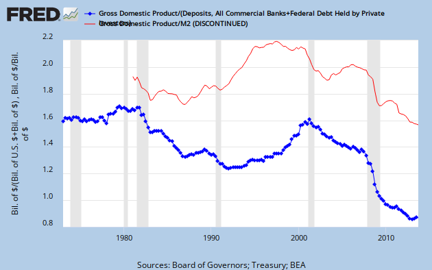 |
| Figure. 5. Money Supply Velocity found from GpMS and M2. |
The Government Provided Money Supply graphs compared to M2 graphs show many differences. These differences can be expected to be the subject of future post on this blog.
No comments:
Post a Comment
Comments are welcomed but are moderated. It may take awhile before they appear to be viewed by all.